Probability Spaces
A lot of systems are very complex. For example describing the motion of water molecules or the stock market. In such cases, it can be impossible to describe the system in such great detail to predict specific outcomes. Instead, we use probabilistic models to describe the system. These probabilistic models use and follow the rules of probability theory.
Another example of a complex system is quantum theory. For most already the name is enough to make them shiver. But in 1900 Max Planck came up with some building blocks to describe the system of quantum theory using probability theory. This was the birth of quantum theory. This was highly controversial at the time because physicists were used to deterministic models, i.e models that were able to predict outcomes with certainty. Einstein was one of the most vocal critics of quantum theory. He famously said “God does not play dice with the universe” and one of his life goals was to find a deterministic model for quantum theory. But so far no one has been able to do so.
These probabilistic models are based on the concept of a probability space, a mathematical model that describes the possible outcomes of a random experiment and the probability of each outcome. A probability space consists of three components:
- A sample space \(\Omega\) which is the set of all possible outcomes of the random experiment.
- An event space \(\mathcal{F}\) which is a collection of events that we are interested in.
- A probability measure \(\P\) which assigns a probability to each event in the event space.
This triplet is called a probability space and is denoted by \((\Omega, \mathcal{F}, \P)\).
Random Experiments
First we need to define what a random experiment is. A random experiment or also called trial is an experiment that can be repeated arbitrarily often and leads to a mutually exclusive and exhaustive set of outcomes.
What does this mean? Mutually exclusive outcomes means that only one of the outcomes can happen at a time. Two outcomes can not happen at the same time. Exhaustive means that one of the outcomes must happen. There are no other outcomes that can happen and are not in the set of outcomes.
Importantly, the outcome of a random experiment is not predictable with certainty beforehand, there is always some element of randomness involved. This is why it is called a random experiment and is the reason why we need probability theory to describe the system.
Some common examples of random experiments are flipping a coin, rolling a die. (We assume that the coin is fair and the die is fair and there is no cheating involved).
With this knowledge, we could already informally describe a probabilistic model of a coin flip. We could say that there are two possible outcomes: heads or tails and that the probability of each outcome is 0.5. A different probabilistic model for the random experiment of flipping a coin could also be if we include the outcome of the coin landing on its side and giving it a very small probability of happening. We could also use a biased coin that has a higher probability of landing on heads than on tails.
It turns out that flipping a coin isn’t actually fair, i.e the probability of heads and tails isn’t 0.5. You can watch this video by Numberphile to know more. The spanish coin is for example slightly heavier on one side and therefore has a higher probability of landing on that side. The same could be true for certain dice dependin on material and the layout of the face values such as discussed here .
Law of Large Numbers
The interesting thing about random experiments is when you perform the experiment once you can not predict the outcome. But if you perform the experiment multiple times you can predict the outcome with better certaincy. The intuition behind this is rather simple, the more times you perform the experiment the more information you have about the system and the better your able to model it and come up with some statistics about the system. For example, if you threw a weirdly shaped dice once you could not predict the outcome. But if you performed the experiment 1000 times you could possibly predict the outcome with a higher degree of certainty. This is called the law of large numbers.
Sample Space
Now to model a random experiment we first need our first component, a set of all the possible outcomes of the random experiment. This set is the so called the sample space and is denoted by \(\Omega\). The elements of the sample space are the mutually exclusive and exhaustive outcomes of the random experiment which are denoted by \(\omega \in \Omega\) and are also often called elementary events, elementary experiments or states.
We’ve seen that mutually exclusive means that they cannot occur simultaneously. For example a coin cannot land on heads and tails at the same time. So we could formally write our sample space for a coin flip as:
\[\Omega = \{\text{Heads}, \text{Tails}\} \]We’ve also seen that our model should be exhaustive, i.e our sample space should contain all possible outcomes. Depending on how complex the experiment is and how much detail we want to include in our model we can include more or less outcomes. For example, if we want to include the outcome of the coin landing on its side we could write our sample space as:
\[\Omega = \{\text{Heads}, \text{Tails}, \text{Side}\} \]The sample space just needs to be exhaustive for our experiments, for example we could agree that if the coin did happen to land on its side we could just ignore that toss. The number of outcomes in the sample space can vary depending on the random experiment but we will see more about this later.
Events
We have seen that an experiment has a sample space of outcomes. Sometimes we are however interested in groupings of outcomes. For example, if we are rolling a die we might be interested in seeing what the probability is of rolling an even number. This is where so called events come into play. An event is a set of outcomes. In other words, an event is a subset of the sample space \(A \subseteq \Omega\). We can then get the set of all possible events by taking the power set of the sample space \(\mathscr{P}(\Omega)\). By defining a set of events that we are interested in we have our second component of the probability space, the event space \(\mathcal{F}\).
If we have an event \(A\) and we perform a random experiment and the experiment results in the outcome \(\omega\) so \(\omega \in \Omega\).
- We then say if \(\omega \in A\), that the event \(A\) has occurred.
- If \(\omega \notin A\) then the event \(A\) has not occurred.
This then leads to two special events that can easily be defined and interpreted:
- The impossible event is the empty set \(\emptyset\). This corresponds to an event that will never occur as some outcome must occur and there are no outcomes in the empty set.
- The certain/sure/guaranteed event is the sample space \(A=\Omega\). This corresponds to an event that will always occur as some outcome must occur and all outcomes are in event \(A=\Omega\).
We have already defined the sample space for rolling a six-sided die as \(\Omega = \{1,2,3,4,5,6\}\). We can now construct the following events, i.e subsets of the sample space:
- Rolling an even number: \(A=\{2,4,6\}\)
- Rolling a number divisible by 3: \(A=\{3,6\}\)
- Rolling a number greater than 2: \(A=\{3,4,5,6\}\)
- Rolling a seven: \(A=\emptyset\), i.e the impossible event since our die only has numbers from 1 to 6.
- Rolling a number between 1 and 6: \(A=\Omega\), i.e the certain event since we are guaranteed to roll a number from 1 to 6.
Sigma Algebra
In some cases we might not want to consider all possible events such as when we define our event space \(\mathcal{F}\) as the power set of the sample space \(\mathscr{P}(\Omega)\) which is the set of all possible events. We wouldn’t want to do this for example when the sample space \(\Omega\) is very large. As the number of elements in the power set is \(|\mathscr{P}(\Omega)|=2^{|\Omega|}\). In such cases we can define a sigma algebra denoted by \(\F\) which is a specific collection of events that we are interested in. To make sure that all the properties of probability theory hold we need to make sure that the sigma algebra satisfies some specific properties. The first property is intuitive and is that the certain event must be in the sigma algebra so:
\[\Omega \in \F \]Secondly if an event is in the sigma algebra then the complement of that event must also be in the sigma algebra:
\[A \in \F \Rightarrow A^c \in \F \]Lastly if we have some events in the sigma algebra then the union of these events must also be in the sigma algebra:
\[A_1,A_2,... \in \F \Rightarrow \bigcup_{i=1}^{\infty} A_i \in \F \]These properties ensure that the sigma algebra is closed under the operations of complement and union. This is important because we want to be able to calculate the probability of complex events by breaking them down into their elementary parts and combining them using set operations.
If we take our running example of rolling a six-sided die we can define different sigma algebras. The following are some valid sigma algebras:
- \(\F = \{\emptyset, \{1,2,3,4,5,6\}\}\), the smallest sigma algebra
- \(\F = \mathscr{P}(\Omega)\), i.e the power set of the sample space with \(|\F|=2^6=64\) the largest sigma algebra
- \(\F = \{\emptyset, \{1,2\}, \{3,4,5,6\}, \{1,2,3,4,5,6\}\}\)
- \(\F = \{\emptyset, \{1,2\}, \{3,4\}, \{5,6\}, \{1,2,3,4\}, \{1,2,5,6\}, \{3,4,5,6\}, \{1,2,3,4,5,6\}\}\)
The above sigma algebras are all valid because they satisfy the properties of a sigma algebra. The following are some invalid sigma algebras:
- \(\F = \{\emptyset, \{1,2\}, \{3,4,5,6\}\}\), the certain event is not in the sigma algebra
- \(\F = \{\emptyset, \{1,2\}, \{3,4\}, \{5,6\}\}\), the union of the events \(\{3,4\}\) and \(\{5,6\}\) is not in the sigma algebra
- \(\F = \{\{1,2,4,5,6\}\}\), the complement of the event \(\{1,2,4,5,6\}\) is not in the sigma algebra
Properties of Events and the Events Space
The above definition of a sigma algebra also has some consequences for events and the power set of the sample space as it is also fullfills the properties of a sigma algebra.
Because the certain event has to be in the sigma algebra and the complement of an event has to be in the sigma algebra we can see that the sigma algebra must therefore also contain the impossible event.
\[\Omega \in \F \Rightarrow \emptyset \in \F \text{ because } \Omega^c = \emptyset \]We have seen in the definition of a sigma algebra that the infinite union of events must also be in the sigma algebra. This general case can also be applied to finite unions of events for example if we have two events \(A\) and \(B\) in the sigma algebra then the union of these events must also be in the sigma algebra.
\[A,B \in \F \Rightarrow A \cup B \in \F \]The proof of this is rather simple as we already have the general case and we know that the empty set is in the sigma algebra. The idea is then that we just add the empty set to the union of the two events infinitely many times to again get to the general case. However, taking the union of the empty set with any set is just the set itself. So we can write the union of two events as:
\[A \cup B = A \cup B \cup \emptyset \cup \emptyset \cup \emptyset \cup \ldots \]So we know that the union of two events is in the sigma algebra but what about the intersection of two events? We can see that the intersection of two events is the complement of the union of the complements of two events. To see this I recommend drawing a Venn diagram.
\[A \cap B = (A^c \cup B^c)^c \]So because the compliment of an event and the union of two events have to be in the sigma algebra and therefore then again its complement we can see that the intersection of two events must also be in the sigma algebra.
\[A,B \in \F \Rightarrow A \cap B \in \F \]Using the general case for the infinite union of events we can also see that the intersection of infinitely many events must also be in the sigma algebra.
\[A_1,A_2,... \in \F \Rightarrow \bigcap_{i=1}^{\infty} A_i \in \F \text{ because } \bigcap_{i=1}^{\infty} A_i = \left(\bigcup_{i=1}^{\infty} A_i^c\right)^c \]Interpretations of Events
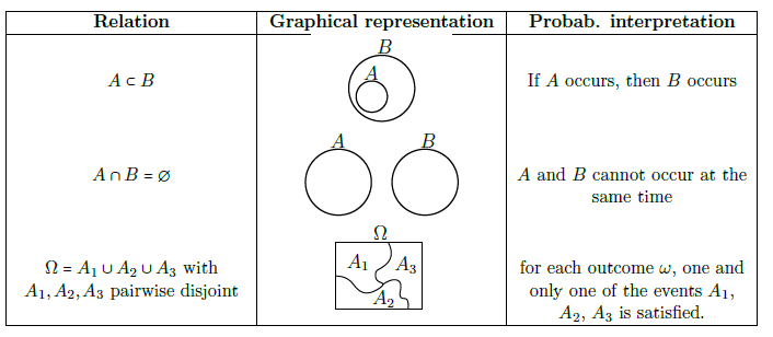
We have seen that events are sets of outcomes and that we can perform operations on these events like unions, intersections and complements.
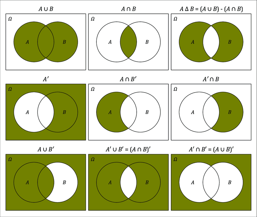
A lot of these events can be visualized and then also interpreted in natural language.
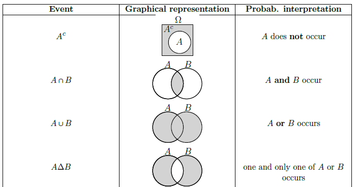
The same goes for the relations between events.
De Morgan’s Laws
One special interaction and interpretation is missing in the above images and that is De Morgan’s laws.
However, it probably makes the most sense to have this in combinatorics as it is more of a combinatorial identity than a probability identity. But it is still important and worth mentioning with a probabilistic example?
Probability Measure
So far we actually haven’t seen any probabilities. We have only defined what experiments are and what outcomes and events can occur. We haven’t defined with what probability these outcomes or events occur. This is where the probability measure comes in. The probability measure is a map or function that assigns a probability to each event in the sample space. Each probability is a number between 0 and 1. 1 means that the event is certain to happen and 0 means that the event is impossible. You can also interpret these decimal values as percentages. So a probability of 0.5 means that the event has a 50% chance of happening. More formally we can define the probability measure on a sample space \(\Omega\) and a sigma algebra \(\mathcal{F}\) as:
\[\begin{align*} \P: &\F \to [0,1] &A \mapsto \P(A) \end{align*} \]For such a function to be a probability measure it needs to satisfy some properties just like the sigma algebra to be compatbile with probability theory. These properties are called the Kolmogorov axioms and were introduced by the Russian mathematician Andrey Kolmogorov in 1933. We can see that each event \(A\) is assigned a probability \(\P(A)\) which is a number between 0 and 1 and that 1 means that the event is certain to happen and 0 means that the event is impossible. This leads to the first property that the probability measure must satisfy.
\[\P(\Omega) = 1 \]so the probability of the certain event is 1 as it will always occur.
Countable Additivity
The next property is called countable-additivity or sometimes also \(\sigma\)-additivity. This property states that the probability of the union of mutually exclusive events is equal to the sum of the probabilities of the individual events.
\[\P(A) = \sum_{i=1}^{\infty} \P(A_i) \text{ where } A = \bigcup_{i=1}^{\infty} A_i \text{ and } A_i \cap A_j = \emptyset \text{ for } i \neq j \text{ so a disjoint union} \]This property is very important because it allows us to calculate the probability of complex events by breaking them down into its disjoint parts which at the lowest level are the probabilities of the outcomes.
We can now define the probability measure for the sample space of rolling a six-sided die. We can say that each outcome is equally likely, so the probability of each outcome is \(\frac{1}{6}\). Therefore the probability measure for the sample space is:
\[\P(\{1\}) = \frac{1}{6}, \P(\{2\}) = \frac{1}{6}, \ldots, \P(\{6\}) = \frac{1}{6} \]Using this we can calculate the probability of more complex events by breaking them down into their disjoint parts. For example, the probability of the event “rolling an even number” is:
\[\P(\{2,4,6\}) = \P(\{2\}) + \P(\{4\}) + \P(\{6\}) = \frac{1}{6} + \frac{1}{6} + \frac{1}{6} = \frac{1}{2} \]Which matches our intuition that the probability of rolling an even number is \(\frac{1}{2}\).
Complementary Events
If we know that the probability of an event \(A\) is \(p\) so \(\P(A) = p\) then we can also quickly calculate the probability of the complementary event so if the event \(A\) does not occur then the event \(A^c\) must occur. The probability of the complementary event is then:
\[\P(A^c) = 1 - \P(A) = 1 - p \]The proof of this is rather simple as we can see that the event \(A\) and the event \(A^c\) are mutually exclusive and exhaustive. So together using countable additivity they make up the entire sample space. So we can write:
\[\P(A) + \P(A^c) = \P(\Omega) = 1 \Rightarrow \P(A^c) = 1 - \P(A) \]Union Bound
The union bound is one of the most useful and frequently encountered inequalities in probability theory. It provides a simple, general upper bound on the probability that at least one of several events occurs—even when those events may overlap. This is especially helpful when direct calculation of the probability of a union is complex or when events are not disjoint.
Before introducing the union bound, it’s essential to understand the monotonicity property of probability measures. The monotonicity property also exists in integral calculus and is a fundamental property of probability measures. Monotonicity says that if one event is a subset of another, then its probability cannot be greater:
\[A \subseteq B \implies \P(A) \leq \P(B) \]This makes sense as every outcome that makes \(A\) happen also makes \(B\) happen (but maybe not vice versa), then \(B\) “covers” at least as much as \(A\) does, so its probability cannot be smaller.
Let \(A, B \in \mathcal{F}\) with \(A \subseteq B\). The set \(B\) can be written as the union of two disjoint sets:
\[B = A \cup (B \setminus A) \]By countable additivity,
\[\P(B) = \P(A) + \P(B \setminus A) \]Since probabilities are always non-negative,
\[\P(B \setminus A) \geq 0 \]we have
\[P(A) \leq \P(B) \]We can derive a useful property for the union of two events. If we have two events \(A\) and \(B\), then the probability of their union can be expressed as:
\[\P(A \cup B) = \P(A) + \P(B) - \P(A \cap B) \]However, we can also just take a loose upper bound by ignoring the intersection term:
\[\P(A \cup B) \leq \P(A) + \P(B) \]This holds because probabilities are non-negative, so the intersection term \(\P(A \cap B)\) is always non-negative. This means that the probability of the union of two events is at most the sum of their individual probabilities (when they are disjoint, this is actually an equality). This property is often referred to as the subadditivity of probability measures.
We can now extend this idea to the case of a finite or countably infinite collection of events which may not be disjoint. This then leads to Boole’s Inequality. Which states that the probability of the union of a collection of events is at most the sum of their individual probabilities. So for any collection of events \(A\_1, A\_2, \ldots \in \mathcal{F}\),
\[\P\left(\bigcup_{i=1}^{\infty} A_i\right) \leq \sum_{i=1}^{\infty} \P(A_i) \]This is also called the union bound as it provides an upper bound on the probability of the union of events. This property also holds for a finite number of events as it can be seen as a special case of the infinite case.
\[\P\left(\bigcup_{i=1}^{n} A_i\right) = \P\left(\bigcup_{i=1}^{\infty} A_i\right) \]where for \(i > n\), we set \(A\_i = \emptyset\). Since \(\P(\emptyset) = 0\), the sum remains unchanged.
Let’s prove the union bound by induction. Base case for \(n = 1\):
\[\P(A_1) \leq \P(A_1) \]which is trivially true. So we now assume the union bound holds for \(n\) events as our induction hypothesis:
\[\P\left(\bigcup_{i=1}^n A_i\right) \leq \sum_{i=1}^n \P(A_i) \]and we want to prove it for \(n+1\) events. So we want to show:
\[\P\left(\bigcup_{i=1}^{n+1} A_i\right) \leq \sum_{i=1}^{n+1} \P(A_i) \]First, observe that
\[\bigcup_{i=1}^{n+1} A_i = \left(\bigcup_{i=1}^{n} A_i\right) \cup A_{n+1} \]By subadditivity (from the axioms),
\[\P\left(\left(\bigcup_{i=1}^{n} A_i\right) \cup A_{n+1}\right) \leq \P\left(\bigcup_{i=1}^{n} A_i\right) + \P(A_{n+1}) \]By the induction hypothesis,
\[\P\left(\bigcup_{i=1}^{n} A_i\right) \leq \sum_{i=1}^{n} \P(A_i) \]Therefore,
\[\P\left(\bigcup_{i=1}^{n+1} A_i\right) \leq \sum_{i=1}^{n} \P(A_i) + \P(A_{n+1}) = \sum_{i=1}^{n+1} \P(A_i) \]Thus, the statement holds for \(n+1\), completing the induction.
Suppose we throw a die \(n \geq 2\) times. We want to prove that the probability of seeing more than \(\ell = \lceil 7 \log n \rceil\) successive 1’s is small when \(n\) is large. We can use the union bound to estimate this probability.
To do this, define the event \(A\) as “there exist \(\ell\) consecutive 1’s in the sequence of outcomes.” We can express this event as a union of events \(A_k\), where each \(A_k\) represents the event that the sequence from positions \(k\) to \(k+\ell-1\) (that is, the \(\ell\) throws starting at throw \(k\)) are all 1’s.
For a fixed \(k \in {1, 2, \ldots, n - \ell + 1}\), define
\[A_k = \left\{ \omega : \omega_{k} = \omega_{k+1} = \dots = \omega_{k+\ell-1} = 1 \right\} \]where \(\omega\) is a sequence of length \(n\) representing the outcomes of the die throws.
For example:
- \(A_1\) is the event that the first \(\ell\) throws are all 1’s,
- \(A_2\) is the event that the second to \((\ell+1)\)-th throws are all 1’s,
- \(A_{n-\ell+1}\) is the event that the last \(\ell\) throws are all 1’s.
We subtract \(\ell-1\) from \(n\) so that the last block of \(\ell\) consecutive throws fits within the \(n\) throws. Thus, the event \(A\) can be written as the union:
\[A = \bigcup_{k=1}^{n-\ell+1} A_k \]The events \(A_k\) are not disjoint—for example, a sequence like \((1, 1, 1, \dots)\) will be in multiple \(A_k\). Therefore, we cannot simply sum their probabilities directly. Instead, we use the union bound:
\[\P(A) = \P\left( \bigcup_{k=1}^{n-\ell+1} A_k \right) \leq \sum_{k=1}^{n-\ell+1} \P(A_k) \]Each \(A_k\) is the event that a specific block of \(\ell\) throws are all 1’s. Since each die throw is independent and the probability of rolling a \(1\) is \(\frac{1}{6}\), we have:
\[\P(A_k) = \left(\frac{1}{6}\right)^{\ell} \]for every \(k\). So,
\[\P(A) \leq (n - \ell + 1) \left( \frac{1}{6} \right)^{\ell} \]If we now plug in \(\ell = \lceil 7 \log n \rceil\), we get (using \(n-\ell+1 \leq n\) for a rough upper bound):
\[\P(A) \leq n \left( \frac{1}{6} \right)^{7 \log n} \]Recall that \(a^{b \log n} = n^{b \log a}\), so:
\[\left( \frac{1}{6} \right)^{7 \log n} = n^{7 \log(1/6)} = n^{-7 \log 6} \implies \P(A) \leq n \cdot n^{-7 \log 6} \]As \(n\) grows, this exponent is negative, and so this probability approaches \(0\). That is, the probability of observing more than \(7 \log n\) consecutive 1’s becomes vanishingly small as \(n\) becomes large.
Continuity of Probability Measure
When we work with probability, we often need to deal not just with single events, but with sequences of events that gradually “grow” or “shrink” toward something more complex. This happens especially in real-world situations. For example, in many problems, we approximate complicated events using simpler ones: for example, we might define an event as “something eventually happens,” which we can express as the limit of a sequence of simpler events.
The continuity property of the probability measure is what lets us make rigorous statements about such limits: it tells us that if we take a sequence of events that approach a final event in a natural way, the probability of the sequence also approaches the probability of the final event. In other words, probability behaves well under limits. Specifically we have two important cases:
- Increasing sequence: If \(A\_1 \subseteq A\_2 \subseteq \ldots\), then
- Decreasing sequence: If \(B\_1 \supseteq B\_2 \supseteq \ldots\), then
The intuition behind these results is as follows:
- Increasing: As we take bigger and bigger events (each containing the last), the probability grows. Eventually, it matches the probability of the “ultimate” event (the union of all). Think of \(A_1 \subseteq A_2 \subseteq ...\) as a sequence of “growing regions” in your sample space. The probability measure follows the growth, never skipping or overshooting, and matches the total region in the end.
- Decreasing: As we shrink the events, the probability gets smaller. In the limit, it matches the probability of what’s left after all the shrinkage (the intersection). Each \(B_n\) shrinks, and the limit is the “core” that never gets removed, the intersection.
Add the images for intuition
Like many proofs in probability, the key is to break down complex events into simpler, disjoint pieces. This is crucial because the probability measure is additive on disjoint sets, allowing us to apply the countable additivity axiom directly.
For increasing sequences, we decompose the \(A_n\) into disjoint pieces. So we set \(\tilde{A}_1 = A_1\) and \(\tilde{A}_n = A_n \setminus A_{n-1}\) for \(n \geq 2\). Each \(\tilde{A}_n\) contains what is new in \(A_n\) compared to \(A_{n-1}\). Because the \(A_n\) are increasing, the \(\tilde{A}_n\) are disjoint and cover the entire union of the \(A_n\):
\[\bigcup_{n=1}^\infty A_n = \bigcup_{n=1}^\infty \tilde{A}_n \]By additivity and the definition of limits we can write:
\[\P\left(\bigcup_{n=1}^{\infty} A_n\right) = \sum_{n=1}^{\infty} \P(\tilde{A}_n) = \lim_{N \to \infty} \sum_{n=1}^{N} \P(\tilde{A}_n) = \lim_{N \to \infty} \P(A_N) \]This shows that as you add more and more of the \(A_n\), you approach the full union’s probability.
For decreasing sequences, we use complements and the result from the increasing case. We define \(B_n^c = B_n^c \cup B_{n+1}^c \cup \ldots\) as the complement of \(B_n\). The complements \(B_n^c\) form an increasing sequence:
\[B_1^c \subseteq B_2^c \subseteq \ldots \]This means we can apply the previous result to \(B_n^c\):
\[\P\left(\bigcap_{n=1}^{\infty} B_n\right) = 1 - \P\left(\bigcup_{n=1}^{\infty} B_n^c\right) = 1 - \lim_{n \to \infty} \P(B_n^c) = \lim_{n \to \infty} \P(B_n) \]Inclusion-Exclusion Principle
This is basically a generalization of countable additivity without the need for disjoint events. It is also a very important principle in combinatorics and probability theory. It is often used to calculate the probability of the union of multiple events when they are not disjoint.
If the probabalities are all the same i.e. we have a Laplace experiment then we can use the formula:
\[|\bigcup_{i=1}^{n} A_i| = |A_1| + |A_2| + \ldots + |A_n| - \sum_{i < j} |A_i \cap A_j| + \sum_{i < j < k} |A_i \cap A_j \cap A_k| - \ldots + (-1)^{n+1} |A_1 \cap A_2 \cap \ldots \cap A_n| = \sum_{k=1}^{n} (-1)^{k+1} \sum_{1 \leq i_1 < i_2 < \ldots < i_k \leq n} |A_{i_1} \cap A_{i_2} \cap \ldots \cap A_{i_k}| \]meaning and interpreataion? Show the basic idea for n=2 and n=3.
For larger cases this becomes annoying which is why we then just use booles inquality as an upper bound.
In algorithms and probability this came up a lot in the exercises as programming it needs to be done using dynamic programming and isn’t as simple as just using the formula.
Laplace Experiments
There are some experiments that occur in a very regular manner, which earns them a name. One such experiment is the Laplace experiment. If all outcomes in a random experiment have the same probability of occurring, meaning all outcomes are equally likely, we speak of a Laplace experiment.
For a sample space of size \(|\Omega|=m\) with \(m\) equally likely outcomes, we have a Laplace space. Each outcome \(\omega_i\) has the same probability, known as counting density:
\[P(\{\omega_i\}) = p(\omega_i)= \frac{1}{m} \text{ with } i=1,2,...,m \]Thus, the probability of an event \(A\) is defined as:
\[P(A) = \sum_{\omega_i \in A}{p(\omega_i)} = |A| \cdot \frac{1}{m} = \frac{|A|}{m} \]When rolling a die, all 6 outcomes are equally likely, making it a Laplace experiment.
For each outcome, \(p(\omega_i) = \frac{1}{6}\)
For the event “even number,” \(A = \{2,4,6\}\), the probability is:
\[P(A)=\frac{3}{6} = \frac{1}{2} = 50\% \]Bernoulli Experiment
Another common experiment is the Bernoulli experiment. A Bernoulli experiment is a random experiment with exactly two possible outcomes. This can often be interpreted as a success/hit or failure/miss.
The most simple Bernoulli experiment is flipping a coin. The two possible outcomes are heads or tails. We can also interpret this as a success if we get heads and a failure if we get tails. Another example is rolling a die. We can interpret this as a success if we roll a 6 and a failure if we roll any other number.
Importantly, unlike a Laplace experiment, the probabilities of the outcomes do not necessarily have to be equal. In the the case of flipping a coin this holds and is a laplace experiment if the coin is fair. But if we have a biased coin then the probabilities of the outcomes are not equal.
We can define a Bernoulli experiment as a random experiment with two possible outcomes, which we can denote as “success” and “failure”.
For example, flipping a coin can be a Bernoulli experiment where we define heads as a “success” and tails as a “failure”. If the coin is fair, the probability of getting heads (success) is \(\frac{1}{2}\) and the probability of getting tails (failure) is also \(\frac{1}{2}\). So it is a Laplace experiment as well.
Another example is rolling a die and defining rolling a 6 as a “success” and rolling any other number as a “failure”. If the die is fair, the probability of rolling a 6 (success) is \(\frac{1}{6}\) and the probability of rolling any other number (failure) is \(\frac{5}{6}\). So this is not a Laplace experiment as the probabilities are not equal.
Another example is where an old british lady says that she can taste the difference between whether the milk was poured before the tea or vice versa. She then has some probabilistic model that she can taste the difference with a probability of \(p\) and that she can not taste the difference with a probability of \(1-p\). This is also a Bernoulli experiment as there are only two possible outcomes, tasting the difference or not tasting the difference.
Why use Sigma Algebras?
As already previously mentioned, in some cases when the sample space is very large we might not want to consider all possible events. In such cases we can define a sigma algebra which is a specific collection of events that we are interested in. Let’s see some examples of why we might want to define a sigma algebra.
Finite Sample Space
This is the simplest case. The sample space contains only a finite number of outcomes:
\[\Omega = \{\omega_1,\omega_2,\omega_3,...\omega_n\} \]Where \(n\) is the number of possible outcomes and \(n \in \mathbb{N}\).
We are playing dungeons and dragons and we are rolling a 20-sided die. Then the sample space is:
\[\Omega = \{1,2,3, \ldots, 20\} \]For the events space we can just take the power set of the sample space:
\[\mathcal{F} = \mathscr{P}(\Omega) = \{\emptyset, \{1\}, \{2\}, \ldots, \{20\}, \{1,2\}, \ldots, \{1,2,\ldots,20\}\} \]And because the d20 is fair we have a Laplace experiment with the probability measure:
\[\P(\{\omega_i\}) = p(\omega_i)= \frac{1}{20} \text{ with } i=1,2,...,20 \]Countable Sample Space
Now if we have a sample space that is countably infinite, we can still define a sample space. This means that the sample space contains infinitely many outcomes, but they can be numbered like the natural numbers.
\[\Omega = \{\omega_1,\omega_2,\omega_3,...\} \text{ with } \omega_i \in \mathbb{N} \text{ and } i=1,2,...,\infty \]Importantly the sample space is countable so \(|\Omega|=|\N|\). This is important asdDespite the sample space being infinite we can still define a probability measure for the sample space that still adds up to 1.
We flip a biased coin multiple times. The coin lands on heads with a probability of \(p\) and on tails with a probability of \(1-p\). If we stop flipping the coin when we get tails we can define the sample space as:
\[\Omega = \N = \{1,2,3,...\} \]Where the outcome is the number of flips until we get tails. This could be any natural number and could therefore also go on forever if we are super unlucky and never get tails. The proability that we get tails after \(k\) flips is:
\[p_k = p^{k-1}(1-p) \text{ with } k=1,2,3,... \]As for the first \(k-1\) flips we have to get heads and on the \(k\)-th flip we have to get tails. As the events space we can again just simply take the power set of the sample space and the probability measure is:
\[P(A) = \sum_{k \in A} p_k = \sum_{k \in A} p^{k-1}(1-p) \text{ with } A \in \mathcal{F} \]To show that this is a valid probability measure we let the sum go to infinity and you just have to trust me that my calculus skills are good enough to show that this converges to 1.
\[\sum_{k=1}^{\infty} p_k = \sum_{k=1}^{\infty} p^{k-1}(1-p) = 1 \]Uncountable Sample Space
Now comes the tricky part. Suppose \(\Omega\) is uncountable, i.e. it contains infinitely many outcomes but they can not be numbered like the natural numbers. An example for such a sample space could be the set of all real numbers between 0 and 1. This is an uncountable set because there are infinitely many real numbers between 0 and 1 and they can not be numbered like the natural numbers.
\[\Omega = [0,1] \text{ or } \mathbb{R} \text{ or } \mathbb{R}^n \]This means that the sample space is uncountable and therefore we can not just take the power set of the sample space as the event space. As for some events we can not define a proability meassure that satisfies the properties of a probability measure such as adding up to 1. So in some cases the following will not work:
\[P(A) = \sum_{\omega \in A} p_{\omega} \text{ with } A \in \mathcal{F} \]For uncountable sets, this kind of sum doesn’t work as if we assign a nonzero probability to each individual point they would sum to infinity, and assigning zero to all points gives a total probability of zero which is also not valid. This is why instead we need to use a special sigma algebras to restrict the events space to a collection of events that we are interested in and for which we can define a probability measure.
Think of a droplet of water in a segment \([0,1]\). The sample space is the set of all possible locations of the droplet in the segment. The sample space is uncountable because there are infinitely many real numbers between 0 and 1. So we can not just take the power set of the sample space as the event space. So instead we use a special sigma algebra called the Borel sigma algebra. I Will not go into detail how it is constructed but you need to be aware that we can not just always use the power set of the sample space.
Same goes for the proability measure. We can not just use the counting density as we did for the finite laplace space. Instead we need to use a special probability measure called the Lebesgue measure. This is a special probability measure that is defined on the Borel sigma algebra and is used to define the probability of events in uncountable sample spaces.